Mastering industrial and commercial lighting calculations is the critical dividing line between a facility that operates safely for decades and one that faces catastrophic compliance failures within its first eighteen months. Relying on guesswork, outdated thumb rules, or simplified wattage-per-square-foot estimations inevitably leads to severe visual discomfort, costly OSHA violations, or bloated capital expenditures.
This comprehensive engineering guide deconstructs the exact mathematical formulas, environmental variables, and thermal limitations that dictate real-world photometric performance. By understanding the underlying physics and commercial variables, procurement teams and facility engineers can move from rough estimates to precise, audit-proof lighting blueprints that optimize both initial investment and long-term maintenance costs.
The Fundamental Fork: Which Lighting Formula Do You Actually Need?
Before you even touch a calculator or begin punching numbers into a spreadsheet, you must define the physical boundaries and characteristics of your target space. In the realm of professional industrial and commercial lighting design, there is no universal, “one-size-fits-all” equation. The presence—or complete absence—of reflective surfaces such as walls, ceilings, and floors fundamentally dictates your entire mathematical approach.
Using the wrong framework is the most common reason projects fail on paper before procurement even begins. We must shatter the simplistic dichotomy that treats all lighting scenarios equally and define the exact optical mechanics at play.
The Standard Dichotomy: Indoor vs. Outdoor Methodologies
To achieve mathematical accuracy, the lighting industry splits baseline calculations into two distinct methodologies based on how light behaves in a given environment. Understanding the difference between these two paths is the absolute foundation of professional photometric design.
- Indoor Spaces (The Lumen Method): Also formally known as the Zonal Cavity Method. This formula is strictly utilized when an environment features enclosing structures—walls, a ceiling, and a floor—that capture and bounce light back into the primary working plane. Its primary function is to calculate the total number of luminaire fixtures required to achieve an average, uniform lux level across a broadly defined area. It relies heavily on measuring how much light is lost to spatial absorption.
- Outdoor Spaces (Point-by-Point Method): This method is deployed when there are no enclosing structural surfaces to reflect light, such as in open parking lots, street lighting grids, or exterior building facades. Because light energy dissipates infinitely into the void of the night sky, this method relies on the Inverse Square Law to calculate the exact lux level at a specific, pinpoint coordinate relative to a single light source or an overlapping array of sources.
Engineering Edge Cases: Navigating the Gray Zones
While the standard dichotomy provides a solid baseline, real-world industrial engineering rarely adheres strictly to black-and-white rules. Veteran lighting designers understand that blindly applying these formulas based merely on whether a space has a roof can lead to disastrous miscalculations. There are critical, high-risk gray zones where the formulas must cross over.
Trap 1: Narrow Aisle High-Bay Warehousing. This is a classic engineering pitfall. While a warehouse is technically an indoor space with walls and a ceiling, the towering, densely packed storage racks completely block light from bouncing off the distant walls or the floor. Furthermore, the critical visual task for forklift operators is not on the floor, but vertically along the rack labels. In this scenario, while you may use the Lumen Method for a rough total fixture baseline, you are forced to utilize the Point-by-Point method to verify vertical illumination uniformity and prevent dangerous shadows.
Trap 2: Heavy Machinery Obstruction. In a sprawling facility, calculating a perfect average horizontal lux is useless if the floor is covered by 4-meter tall CNC machines or massive stamping presses. The Lumen Method assumes an “empty cavity.” The shadows cast by these machines will turn critical operating stations into dark zones. The standard calculation must be heavily penalized, and task lighting integrated.
Trap 3: Exterior Canopies and Gas Stations. Conversely, a gas station canopy or a loading dock overhang is located outdoors. However, it features a massive, highly reflective ceiling structure directly above the working plane. Because of this trapped, concentrated reflectance, engineers can successfully adapt the Lumen Method to estimate the total required lumen package, rather than strictly calculating point-by-point grids from the outset.
Indoor Mastery: The Lumen Method and Its Critical Variables
The standard equation for achieving uniform indoor general lighting is written as:
N = (E × A) / (Φ × CU × LLF)
In this fundamental formula, N represents the total number of fixtures required, E is the target illuminance in Lux, A is the total area in square meters, and Φ represents the initial lumen output of a single fixture.
While the numerator (Target Lux × Area) represents your raw optical demand, the true engineering challenge lies entirely in the denominator. Failing to accurately assess the environmental variables—specifically the Coefficient of Utilization (CU) and the Light Loss Factor (LLF)—will result in calculating a system that looks perfect in a theoretical vacuum, but rapidly degrades into a dark, non-compliant hazard in physical reality.
Room Cavity Ratio (RCR): The Prerequisite to CU
Before you can possibly determine how much light your specific walls will absorb, you must first calculate the volumetric, three-dimensional proportions of the space. This is a crucial step that amateurs frequently skip. A 20-meter high, incredibly narrow deep-well heavy manufacturing plant and a 5-meter high, sprawling open assembly floor might be painted with the exact same white reflective epoxy, but their geometric light loss is drastically different. The deep well will swallow and trap light laterally long before it ever reaches the working floor.
To quantify this geometry, optical engineers use the Room Cavity Ratio (RCR) formula:
RCR = [5 × Height of cavity × (Length + Width)] / (Length × Width)
The resulting number (typically falling between 1 and 10) serves as your primary spatial index. Only after calculating your specific RCR can you intelligently consult a luminaire manufacturer’s IES (Illuminating Engineering Society) photometric data sheet to extract the correct utilization percentage for your unique project.
Coefficient of Utilization (CU): Accounting for Reflectance
The Coefficient of Utilization (CU) is a decimal representation of the percentage of total lumens emitted by the fixtures that actually reach the defined work plane after bouncing off the ceiling, walls, and floor. It sits securely in the denominator of our core equation for a critical mathematical reason: a lower CU mathematically forces the equation to output a higher number of required fixtures to compensate for the light lost to the room’s surfaces.
To find your precise CU, you take your calculated RCR and cross-reference it with the reflectance values of your room. In the commercial industry, these are standardly expressed in ratios like 80/50/20 (which denotes 80% ceiling reflectance, 50% wall reflectance, and 20% floor reflectance).
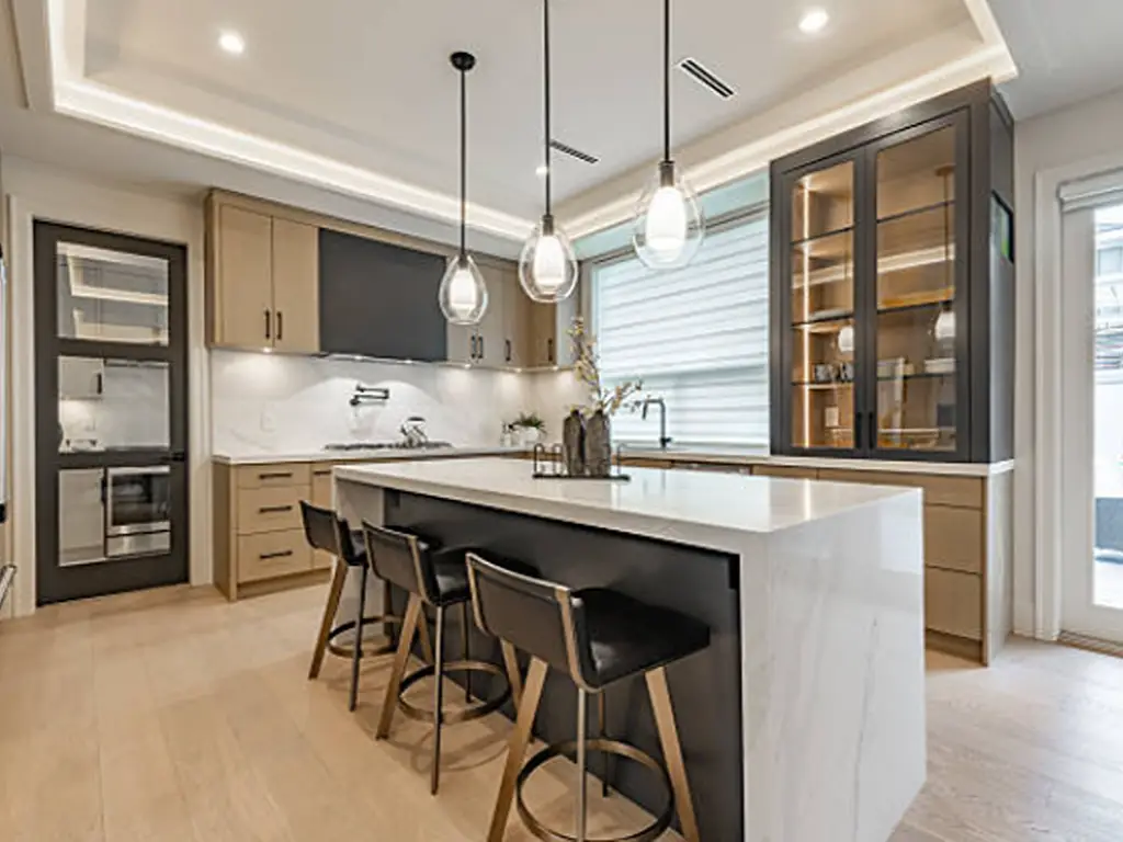
A pristine corporate office environment with white drop ceilings will yield a high CU (e.g., 0.85), meaning 85% of the purchased light is efficiently utilized. Conversely, a heavy forging facility with dark, soot-covered walls and an exposed black steel ceiling might yield a CU of 0.45. This means over half of the optical energy you purchase is instantly wasted by spatial absorption, forcing you to double your fixture count simply to hit the baseline target.
Dissecting the Light Loss Factor (LLF) & The Harsh Environment Cheat Sheet
If CU accounts for the fixed geometry of the space, the Light Loss Factor (LLF) is the dynamic, engineered redundancy required to future-proof your lux levels against the relentless march of time, dirt, and thermal decay. If you calculate your facility using an LLF of 1.0, you are designing a lighting system that will only meet legal safety standards on the absolute first day it is turned on.
Real-world LLF is not a random safety margin guessed by a contractor; it is the multiplied product of several harsh physical realities. An accurate LLF must synthesize multiple degradation metrics:
- Lumen Depreciation (LLD): This accounts for the inevitable degradation of the LED chip and its phosphor coating over tens of thousands of operating hours. As the diode ages, its quantum efficiency naturally diminishes.
- Luminaire Dirt Depreciation (LDD): This variable represents the accumulation of airborne particulates, industrial grease, and dust on the optical lenses of the fixtures, which physically obstruct and scatter light from escaping the housing.
- Ambient Temperature Factor (The Silent Killer): This is a frequently overlooked, yet completely fatal parameter in B2B heavy industry. LEDs are highly thermally sensitive semiconductor components. As ambient environmental heat rises, junction temperature spikes, and semiconductor efficiency drops. If you install standard fixtures in a 50°C steel mill roof environment, the actual lumen output will instantly experience thermal derating, often dropping by 15% or more from its laboratory-rated nominal value.
The Industrial Environment LLF Cheat Sheet:
To eliminate the guesswork when building your optical formulas, use these industry-standard baseline estimates for Dirt Depreciation and total LLF based on specific facility conditions:
- Clean / Climate Controlled (Laboratories, Clean Warehouses): LDD can be safely estimated at 0.85. The environment poses minimal threat to the sealed optics.
- Normal Manufacturing (Assembly Lines, General Processing): LDD should drop to 0.75. Standard particulate suspension will gradually coat the lenses over a standard two-year maintenance cycle.
- Heavy Harsh Environments (Welding Shops, Foundries, Heavy Machining): LDD must be aggressively penalized down to 0.65 or lower. The presence of heavy oil mist, metallic dust, and high heat requires you to mathematically over-engineer the initial fixture count by over 30% simply to ensure the facility remains legally compliant after eighteen months of operational abuse.

Outdoor & Precise Task Lighting: The Point-by-Point Method
When you move outside the walls of a facility, the Lumen Method entirely collapses. Without walls or ceilings to bounce light back to the ground, light energy dissipates geometrically outward into the atmosphere. To calculate outdoor parking areas, streetscapes, or pinpoint industrial task lighting, engineers must transition to the Point-by-Point Method, which is governed strictly by the laws of optical physics.
However, outdoor environments present their own severe traps. Forgetting to account for extreme weather LDD (like coastal salt spray destroying lens transmissivity) or failing to calculate Light Trespass (BUG rating violations) across property lines can lead to immediate legal injunctions and forced redesigns.
The Inverse Square Reality (E = I / d²)
The absolute core of outdoor photometric calculation is the Inverse Square Law. In this formula, E remains your target Illuminance in Lux. I represents the Luminous Intensity of the light source directed at a specific angle, measured in Candelas (cd). Finally, d represents the direct linear distance from the light source to the target calculation point on the ground.
The vital, uncompromising concept here is the squared distance (d²). This mathematical reality dictates that if you take an outdoor area light and mount it twice as high on a steel pole, the illumination directly beneath it on the asphalt does not simply cut in half—it geometrically collapses to one-quarter of its original intensity. Because the light is spreading over a spherical surface area that grows exponentially as it travels, calculating mast height and fixture wattage becomes an incredibly delicate balancing act to ensure enough usable light reaches the ground to prevent accidents.
The Cosine Law for Angled Illumination
The Inverse Square Law works perfectly if you are calculating the exact spot directly beneath the light fixture (known as the nadir). However, a sprawling logistics parking lot or a municipal roadway requires uniform light across vast stretches of space. When light travels at a diagonal angle to strike the ground further away from the pole base, the beam spreads out over a stretched, elliptical area, drastically reducing its intensity.
To accurately calculate these critical peripheral zones, we introduce the Cosine Law of Illuminance:
E = (I / d²) × cos(θ)
Here, θ (theta) represents the angle of incidence between the light beam and the perpendicular normal line of the ground. As the angle increases (meaning you are attempting to illuminate a spot further away from the pole), the cosine value drops, plummeting the lux level. This precise calculation dictates exactly how far apart you can space your streetlights or high-mast poles before the optical overlap fails and hazardous, liability-inducing “dark zones” appear.

Comprehensive Industry Lux Standards (Backed by IESNA & EN 12464-1)
A mathematical formula is utterly useless if you do not know what target value to insert into the E (Target Lux) variable. In the B2B industrial and commercial sectors, setting this target is not a matter of subjective preference or guessing; it is a matter of strict legal compliance, operational efficiency, and occupational safety. Designing a facility below recognized optical thresholds exposes the enterprise to severe OSHA audit risks, increased accident liability, and drastic, unrecoverable losses in worker productivity.
The following foundational targets are anchored directly in the authoritative recommendations of the EN 12464-1 European Standard for Workplace Lighting and North American IESNA (Illuminating Engineering Society of North America) guidelines. These figures serve as your legally defensible baseline for inserting variables into either the Lumen or Point-by-Point equations.
| Application Environment | Recommended Target (E) | Hardcore Standard Reference |
|---|---|---|
| Heavy Machining / Rough Assembly | 300 – 500 Lux | EN 12464-1 |
| Precision Manufacturing / Quality Inspection | 750 – 1000+ Lux (High CRI Required) | IESNA / EN 12464-1 |
| High-Bay Warehousing (Open Floor Layout) | 150 – 200 Lux | IESNA |
| Outdoor Parking Lots (General Active) | 20 – 50 Lux (Minimum Uniformity Limits Apply) | IESNA RP-20 |
| Corridors, Walkways, and Stairs | 100 – 150 Lux | EN 12464-1 |
The Interactive B2B Lighting Requirement Calculator
To bridge the gap between abstract physics and practical project planning, we have engineered an interactive calculation matrix. This tool allows procurement teams and facility engineers to seamlessly input their spatial dimensions and manipulate the critical environmental variables discussed above.
By adjusting the operational environments, you can instantly visualize how the Coefficient of Utilization and Light Loss Factors mandate severe shifts in your total fixture requirements. Crucially, this calculator embeds Professional Edge Case Logic. If you input hazardous variables—such as towering narrow racks, heavy machinery obstructions, or extreme outdoor cosine angles—the calculator will automatically apply the necessary derating coefficients or hard-stop the calculation to prevent dangerous safety violations.
Engineering Formula Simulator

Total Cost of Ownership (TCO): Why Hardware Dictates Formula Accuracy
Calculations and mathematical formulas are inherently theoretical. You can spend weeks perfectly mapping out a massive manufacturing facility, meticulously calculating a Light Loss Factor of 0.65, and precisely modeling the Coefficient of Utilization to ensure absolute compliance. However, if the procurement phase results in the installation of poorly engineered, commoditized hardware, the physical reality will immediately betray your mathematical models.
Total Cost of Ownership (TCO) in industrial lighting is fundamentally divided into Initial Capital Expenditure (CAPEX) and long-term Operational Expenditure (OPEX). While many procurement buyers hyper-focus on the cheapest initial fixture price, true engineering disasters occur in the OPEX phase. When cheap lighting systems fail prematurely due to thermal overload, facility managers are forced to halt lucrative production lines, hire specialized union contractors, and rent expensive heavy machinery, such as $1,000-a-day scissor lifts, simply to reach and replace degraded high-bay fixtures at the ceiling level. This recurring maintenance nightmare completely obliterates any perceived savings from cheap hardware.
Formulas assume stable hardware. If your LED’s junction temperature exceeds its physical limits, Lumen Depreciation accelerates exponentially, rendering your Year 1 calculations entirely invalid by Year 2.
At WOSEN LED, we structurally lock in your thermal parameters to ensure your calculated Light Loss Factor never collapses under real-world stress. Instead of relying on fragile active cooling mechanisms (like internal fans) that frequently clog and fail in high-dust industrial environments, our heavy-duty fixtures utilize advanced passive thermal management driven by optimized, pure die-cast aluminum heat sinks.
This extreme heat dissipation framework actively pulls heat away from the diode, keeping LED junction temperatures well below critical failure limits, even in punishing 50°C ambient manufacturing environments. This fundamentally prevents the catastrophic lumen depreciation that destroys TCO calculations.
We do not merely promise “calculation-true optics.” We back our engineering integrity with third-party certified LM-79 (photometric distribution) and LM-80/TM-21 (lumen maintenance lifespan) test reports. Your facility calculations remain firmly anchored in IESNA-recognized laboratory data, providing an absolute audit trail for compliance. Furthermore, our proprietary, automated factory-direct manufacturing model entirely eliminates middleman markups, effectively absorbing the initial CAPEX shock and delivering premium, reliable optical performance at an uncompromised value.
Conclusion: Validating Your Calculation with 3D Simulation
Understanding the core mathematical formulas, whether applying the Lumen Method to account for complex indoor geometric reflectance or utilizing the Point-by-Point inverse square law for expansive outdoor grids, is the irreplaceable first step in professional lighting design. These calculations empower you to establish accurate budgets and definitively prove baseline compliance to stakeholders.
However, manual equations are ultimately baseline estimations. They cannot account for physical obstructions, complex machinery shadowing, or intricate glare ratings (UGR). Before committing millions to procurement, these mathematical frameworks must be validated against physical reality to prevent spatial anomalies.
Always transition your mathematical findings into professional, software-driven 3D simulations utilizing certified IES photometric data. This transition from formula to simulation guarantees flawless operational execution, ensuring that the light you calculated on paper is exactly the light that hits the factory floor.
Ready to Prove Your Calculations?
Don’t leave compliance to chance. Send us your facility dimensions, and our engineering team will transition your manual calculations into a comprehensive, highly accurate 3D DIALux simulation—completely free of charge.
Request Your Free 3D Simulation Today